SEP fluence model

This calculation tool models solar energetic particle (SEP) fluence at very high energies. Based on pre-calculated tabulated model data, the tool interpolates the fluence for a user-specified mission length. Depending on the mode of operation, the user can also choose from other model parameters, as described in the user instructions below.

The model is based on an analysis of ground level enhancements (GLEs) and sub-GLEs between April 1976 and December 2017. Here sub-GLEs refer to events that have been observed above 300 MeV, but have not produced sufficient intensities at higher energies to be observed on ground. Tylka and Dietrich (2009) showed that the integral proton fluence spectrum of a GLE event at energies above 10 MeV can be represented by a double power law in rigidity with a smooth roll-over from one power law at low rigidities to the other at the highest rigidities. The fit function (Band et al., 1993) contains four parameters: the two spectral indices γ₁ and γ₂, the breakpoint rigidity R₀ and the fluence normalization factor J₀. The GLE spectral analysis was extended into the sub-GLEs by Atwell et al. (2016). More recently, Koldobskiy et al. (2021) revised the GLE spectra using an updated neutron monitor yield function. They used a modified Band function (MBF) to represent the revised spectra. The MBF differs from the Band function in that it has an additional exponential roll-over at high rigidities; it has five fitted parameters: low and high rigidity spectral indices γ₁ and γ₂, low and high turnover rigidities R₁ and R₂, and the high rigidity fluence normalization factor J₂.

This model is based on the Band function representations of sub-GLEs and the modified Band function representations of GLEs, with the exception of events too small for the spectral fitting, namely GLE 34, which was calculated using SEPEM RDS v2.2, and GLEs 52, 57 and 68, for which the Band function representations were used. Since the duration of the time integration in the GLE revision was based on very high energies, a significant portion of the fluence at low or medium energies was not covered. To correct for this, the spectra of GLEs 43 and 58 were supplemented with Tylka's separately analysed ESP components, and the spectra of GLEs 51, 59 and 62 with integral GOES fluxes. The parameters of the Band function and modified Band function representations can be found in Vainio et al. (2017), Raukunen et al. (2018) and Koldobskiy et al., (2021).

Our initial dataset spans 46 GLEs and 64 sub-GLEs. The earlier sub-GLEs are observed with IMP and the later with GOES/HEPAD, and the background of GOES/HEPAD is much higher than the background of IMP. To make the dataset homogenous we omit the IMP-observed sub-GLEs with >433 MeV fluences smaller than 10² cm^-2 sr^-1, which could not have been observed with GOES/HEPAD. This leaves us with a dataset of 46 GLEs and 46 sub-GLEs.

Analysing the waiting times of GLEs and sub-GLEs reveals that closely spaced events are not occurring randomly. However, by combining closely spaced events emitted by the same active region at the Sun to single episodes (containing 1-5 events) the random character of the occurrence is recovered and the episode occurrence can be modelled as a Poisson process.

Episode fluences are calculated by summing the fluence spectra of the events belonging to the episode. Then, fluence distributions are constructed by sorting the episode fluences by increasing size and assigning them probabilities proportional to their rank, individually for each of the logarithmically spaced energies of the model. These distributions are then fitted with exponentially cut-off power law functions.

The fluence modelling was done by modelling the number of SEP episodes for a specified mission duration with a Poisson distribution. Then, for each episode, the episode fluences were modelled using the cut-off power law distributions. The largest episode fluence for each energy channel is taken as the worst-case fluence and the sum of episode fluences as the cumulative fluence, and the process is repeated until a desired statistical accuracy is reached. This Monte Carlo simulation is performed for missions of various durations and for each duration the cumulative fluence and the worst-case fluence is tabulated for different confidence levels, yielding the raw data of the model.

A careful analysis of the occurrence of the events shows that waiting times longer than 700 days are not well-described by a Poisson process. This can be shown to be due to solar minimum activity periods, which make the long waiting times more probable than predicted by a single Poisson process. Therefore, the tool also offers a two-component model that breaks the solar activity cycle into 7 active and 4 quiet years, and considers a different event rate for each. We recommend to use the two-component model for missions longer than 2 years and/or occurring outside the solar maximum period.

User instructions

SEP fluence probability calculator

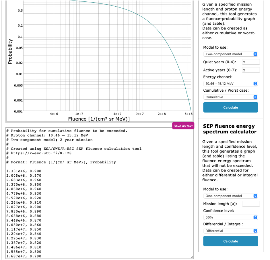
This tool calculates the probability of exceeding a fluence on a mission of a given length. The user can specify whether to use the one-component model (single Poisson process) or the two-component model (active and quiet years separated), give the mission duration (or the number of active and quiet years for the two-component model), choose the energy channel from thirteen options and specify, whether the tool should output cumulative fluences over the whole mission or the worst-case event fluences as the abscissa value. The values of mission length should be between 0.5 and 7 years for the one-component model, and duration between 0.5 and 11 years (with 0-7 active years and 0-4 quiet years) for the two-component model, to ensure functionality of calculator.

When using valid parameters (for example two-component model, 2 active years and 2 quiet years, energy channel 10.46-15.12 MeV and cumulative model), the result should look like this

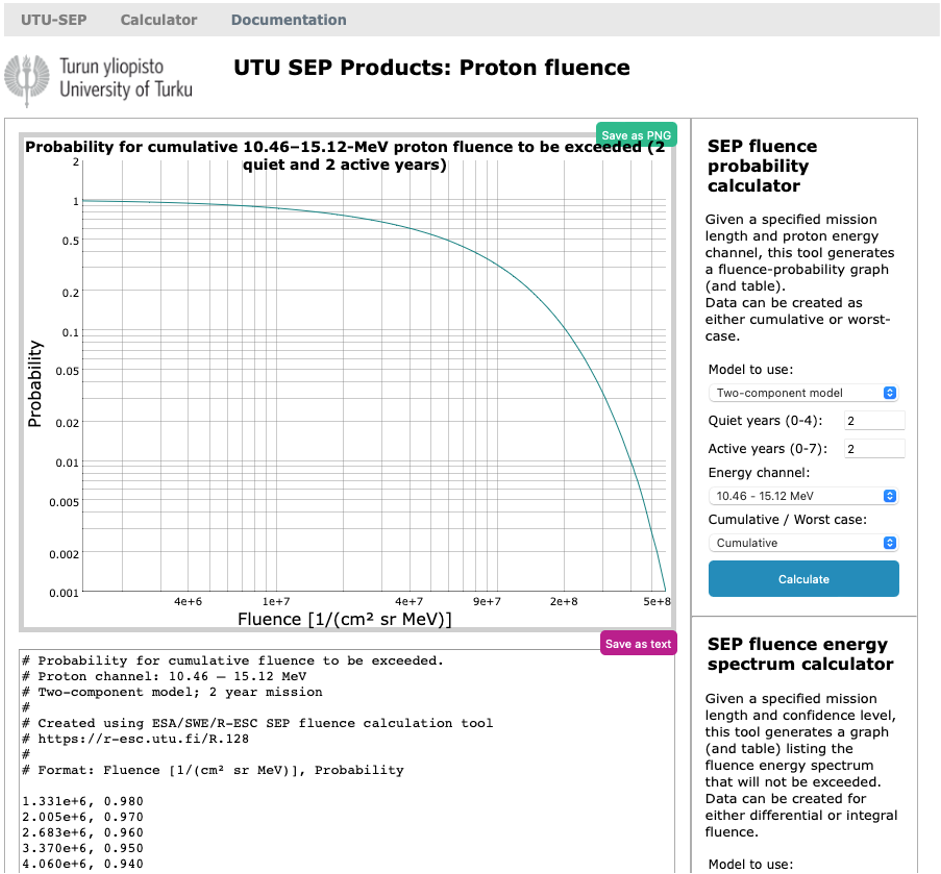
The user can hover over the plot area and read the values of the points closest to the cursor on the screen. The plot, once created, can also be saved as a PNG file using the button on the right. Alternatively, the raw data of the plot in numeric format can be copied and pasted out from the text field below the plot area.

In case you click the green button to save the PNG file, the image appears in a new window:

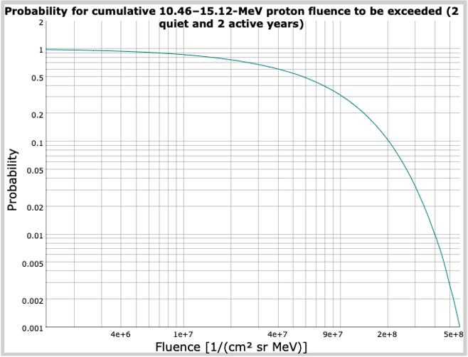
You can then right-click on it and choose to save it in a file.

SEP fluence energy spectrum calculator

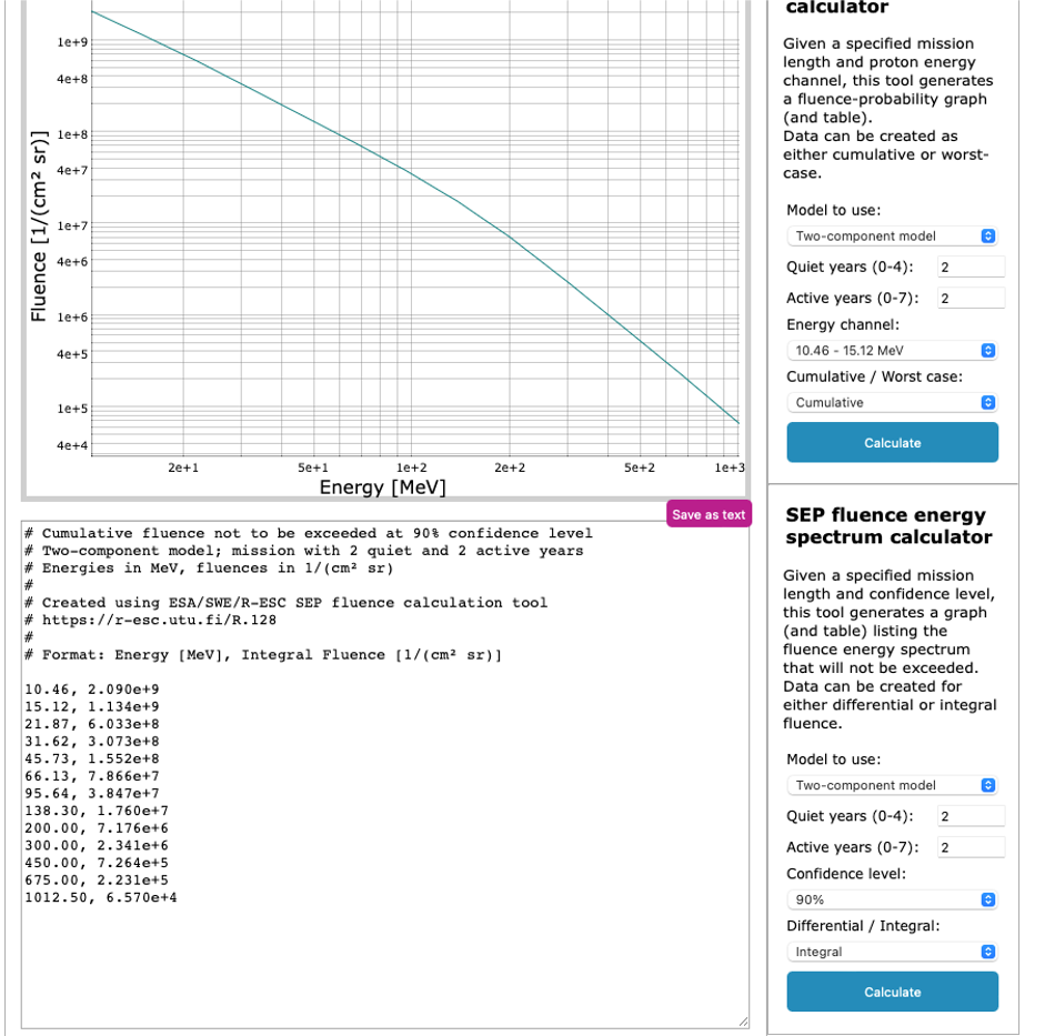
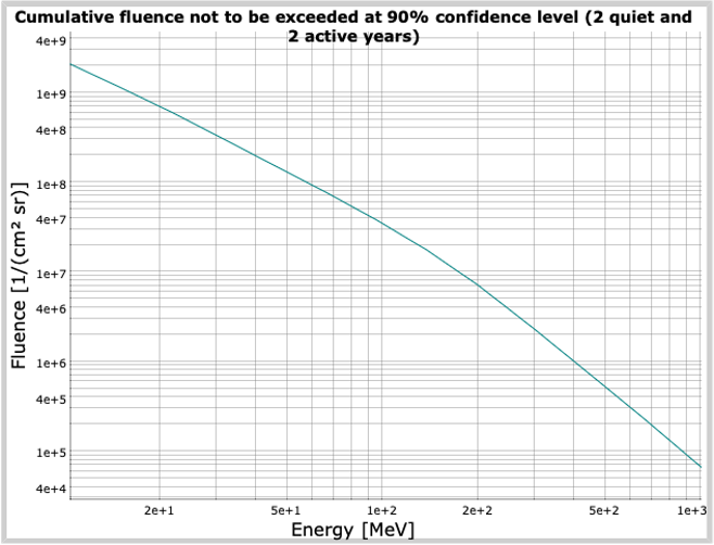
This tool calculates the energy spectrum of the cumulative fluence not to be exceeded during the mission. The user can specify whether to use the one-component model (single Poisson process) or the two-component model (active and quiet years separated), give the mission duration (or the number of active and quiet years for the two-component model), choose the confidence level from four options (50%, 90%, 95%, and 99%) and specify, whether the tool should output differential or integral fluences. The values of mission length should be between 0.75 and 7 years for the one-component model, and the number of active years between 0.75-7 and quiet years between 0-4 for the two-component model, to ensure functionality of calculator.

The tool gives differential fluence as a function of average of channel limits as the abscissa and integral fluence as a function of the lower limit of the energy channel. An example of such a fluence energy spectrum (two-component model, 2 active years and 2 quiet years, confidence level 90%, and integral fluence) is given below:

Machine-to-machine interfaces

The machine-to-machine interface (API) to the product is provided as a web page located at

https://r-esc.utu.fi/api/R.128/<calculator_type>?model=<fluence_model>&<parameter_list>

Here <calculator_type> is either the string ‘probability’ or the string ‘energy’ for accessing the probability calculator or the energy spectrum calculator, respectively; <fluence_model> is either the string ‘onecomponent’ or the string ’twocomponent’ for using the one-component or the two-component model; and the <parameter_list> depends on the chosen product variant, as explained below. In all cases the output of the API is a csv file identical to the GUI except for the header part, which is omitted.

The probability calculator one-component fluence model has three parameters in addition to the fluence model.

Parameter name	Type	Range / allowed values	Description
mission_length	float	0.5 — 7.0	Mission duration in years
energy_channel	integer	1 — 13	Energy channel (see below for corresponding MeV values)
mode	string	“cumulative” or “worstcase”	Output mode selector between cumulative fluences and worst-case event fluences.

energy_channel value index correspondence to energy value:

energy_channel	Description
1	10.46 — 15.12 MeV
2	15.12 — 21.87 MeV
3	21.87 — 31.62 MeV
4	31.62 — 45.73 MeV
5	45.73 — 66.13 MeV
6	66.13 — 95.64 MeV
7	95.64 — 138.3 MeV
8	138.3 — 200.0 MeV
9	200.0 — 300.0 MeV
10	300.0 — 450.0 MeV
11	450.0 — 675.0 MeV
12	675.0 — 1012.5 MeV
13	> 1012.5 MeV

For example, acquiring the cumulative fluence probability distribution in energy channel 12 for a three-year mission using the one-component model, access the following web page:

https://r-esc.utu.fi/api/R.128/probability?model=onecomponent&mission_length=3.0&energy_channel=12&mode=cumulative

The probability calculator two-component fluence model has four parameters in addition to the fluence model.

Parameter name	Type	Range / allowed values	Description
quiet_years	float	0.0 — 4.0	Number of quiet years of solar activity
active_years	float	0.0 — 7.0	Number of active years of solar activity
energy_channel	integer	1 — 13	Energy channel (see below for corresponding MeV values)
mode	string	“cumulative” or “worstcase”	Output mode selector between cumulative fluences and worst-case event fluences

The sum of quiet_years + active_years must greater than 0.5.

energy_channel value index correspondence to energy value:

energy_channel	Description
1	10.46 — 15.12 MeV
2	15.12 — 21.87 MeV
3	21.87 — 31.62 MeV
4	31.62 — 45.73 MeV
5	45.73 — 66.13 MeV
6	66.13 — 95.64 MeV
7	95.64 — 138.3 MeV
8	138.3 — 200.0 MeV
9	200.0 — 300.0 MeV
10	300.0 — 450.0 MeV
11	450.0 — 675.0 MeV
12	675.0 — 1012.5 MeV
13	> 1012.5 MeV

For example, acquiring the worst-case fluence probability distribution in energy channel 10 using the two-component model a mission with two active and one in-active year, access the following web page:

https://r-esc.utu.fi/api/R.128/probability?model=twocomponent&quiet_years=1.0&active_years=2.0&energy_channel=10&mode=worstcase

The energy spectrum calculator one-component fluence model has three parameters in addition to the fluence model.

Parameter name	Type	Range / allowed values	Description
mission_length	float	0.75 — 7.0	Mission duration in years
confidence	string	“50”, “90”, “95” or “99”	Confidence level in percentages
mode	string	“differential” or “integral”	Output mode selector between differential and integral fluences

For example, acquiring the differential energy spectrum of the fluence at 90% confidence level using the one-component model for a four-year mission, access the following web page:

https://r-esc.utu.fi/api/R.128/energy?model=onecomponent&mission_length=4.0&confidence=90&mode=differential

The energy spectrum calculator two-component fluence model has four parameters in addition to the fluence model.

Parameter name	Type	Range / allowed values	Description
quiet_years	float	0.0 — 4.0	Number of quiet years of solar activity
active_years	float	0.75 — 7.0	Number of active years of solar activity
confidence	string	“50”, “90”, “95” or “99”	Confidence level in percentages
mode	string	“differential” or “integral”	Output mode selector between differential and integral fluences

For example, acquiring the integral energy spectrum of the fluence at 95% confidence level using the two-component model for a mission of 2.0 quiet years and 3.0 active years, access the following web page:

https://r-esc.utu.fi/api/R.128/energy?model=twocomponent&quiet_years=2.0&active_years=3.0&confidence=95&mode=integral

References

Atwell W. et al., 2016, In Proc. 46th International Conference on Environmental Systems
Band D. et al., 1993, Astrophysical Journal, 413, 281
Koldobskiy S. et al., 2021, Astronomy & Astrophysics, 647, A132
Raukunen, O. et al., 2018, Journal of Space Weather and Space Climate, 8, A04
Tylka A.J. and Dietrich W.F., 2009, In Proc. 31st International Cosmic Ray Conference
Vainio R. et al., 2017, Astronomy & Astrophysics, 604, A47